Tutorial 6: 3D Mouse Brain

Load the Mouse Brain

import scanpy as sc
import pandas as pd
import numpy as np
import matplotlib.pyplot as plt
import sys
import os
import gc
import warnings
warnings.filterwarnings("ignore")
sys.path.append('/mnt/mydisk/home/chenxd/FlatST')
import FlatST
import STAGATE_pyG

adata = sc.read_h5ad('/mnt/mydisk/home/chenxd/FlatST/Reply/9/counts_mouse4_sagittal.h5ad')

Processing three-dimensional data

z_coords = {'sa2_slice1': 0, 'sa2_slice2': 20, 'sa2_slice3': 40}
adata.obs['Z'] = adata.obs['slice_id'].map(z_coords).astype(float)
adata.obs['X'] = adata.obs['center_x']
adata.obs['Y'] = adata.obs['center_y']
adata.obs['Section_id'] = adata.obs['slice_id']

# Important: Add spatial coordinates to obsm
adata.obsm['spatial'] = adata.obs[['center_x', 'center_y']].values

# Normalization
sc.pp.highly_variable_genes(adata, flavor="seurat_v3", n_top_genes=3000)
sc.pp.normalize_total(adata, target_sum=1e4)
sc.pp.log1p(adata)

Training

# FlatST 3D Spatial Network
section_order = ['sa2_slice1', 'sa2_slice2', 'sa2_slice3']
keep_cells = adata.obs.notna().all(axis=1)
adata = adata[keep_cells].copy()
FlatST.Cal_Spatial_Net_3D(adata, rad_cutoff_2D=10, rad_cutoff_Zaxis=1,
                           key_section='Section_id', section_order=section_order, verbose=True)

Radius used for 2D SNN: 10
Radius used for SNN between sections: 1
------Calculating 2D SNN of section  sa2_slice1
This graph contains 12254 edges, 43835 cells.
0.2795 neighbors per cell on average.
------Calculating 2D SNN of section  sa2_slice2
This graph contains 18284 edges, 52298 cells.
0.3496 neighbors per cell on average.
------Calculating 2D SNN of section  sa2_slice3
This graph contains 30808 edges, 77716 cells.
0.3964 neighbors per cell on average.
------Calculating SNN between adjacent section sa2_slice1 and sa2_slice2.
This graph contains 358 edges, 96133 cells.
0.0037 neighbors per cell on average.
------Calculating SNN between adjacent section sa2_slice2 and sa2_slice3.
This graph contains 342 edges, 130014 cells.
0.0026 neighbors per cell on average.
3D SNN contains 62046 edges, 173849 cells.
0.3569 neighbors per cell on average.

# Train FlatST - reducing epochs for verification
adata = FlatST.train_FlatST(adata, n_epochs=1000, is_distribution=0.0, num_smooth_iterations=[4,0], cuda_device=4)

# mclust
os.environ['R_HOME'] = '/mnt/mydisk/home/chenxd/.conda/envs/r_env/lib/R'
num_cluster = 15
adata = FlatST.mclust_R(adata, num_cluster, used_obsm='FlatST')

Size of Input:  (173849, 1135)

100%|██████████| 1000/1000 [02:04<00:00,  8.03it/s]

fitting ...
  |======================================================================| 100%

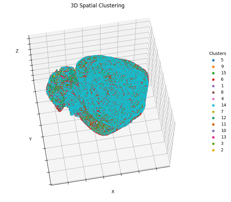
Draw

# Plot 3D clusters
import matplotlib.pyplot as plt
import pandas as pd
import numpy as np

fig = plt.figure(figsize=(8, 8))
ax1 = plt.axes(projection='3d')

# Define a color list containing sufficient colors to match your num_cluster.
adata.uns['mclust_colors'] = ['#1f77b4', '#ff7f0e', '#2ca02c', '#d62728', '#9467bd',
                              '#8c564b', '#e377c2', '#17becf', '#bcbd22', '#1b9e77',
                              '#d95f02', '#7570b3', '#e7298a', '#66a61e', '#e6ab02']

# Get all cluster labels
region_labels = pd.Series(adata.obs['mclust']).dropna().unique().tolist()

for it, label in enumerate(region_labels):
    # Filter out the cells belonging to the current cluster
    temp_Coor = adata.obs.loc[adata.obs['mclust'] == label, :]
    temp_xd = temp_Coor['X']
    temp_yd = temp_Coor['Y']
    temp_zd = temp_Coor['Z']

    # Cycle through the colors in the list to assign colors to the clusters
    color = adata.uns['mclust_colors'][it % len(adata.uns['mclust_colors'])]

    # Plot 3D scatter plot for the current cluster
    ax1.scatter3D(temp_xd, temp_yd, temp_zd, c=color, s=10, marker=".", label=label)

# Hide axis labels to keep the plot clean
ax1.set_xlabel('X')
ax1.set_ylabel('Y')
ax1.set_zlabel('Z')
ax1.set_xticklabels([])
ax1.set_yticklabels([])
ax1.set_zticklabels([])

# Set legend legend and view angle
plt.legend(bbox_to_anchor=(1.2, 0.8), markerscale=3, frameon=False, title="Clusters")
plt.title('3D Spatial Clustering')
ax1.elev = 60  # elevation
ax1.azim = 80 # azimuth

# Show the plot
plt.show()

import scanpy as sc
import matplotlib.pyplot as plt

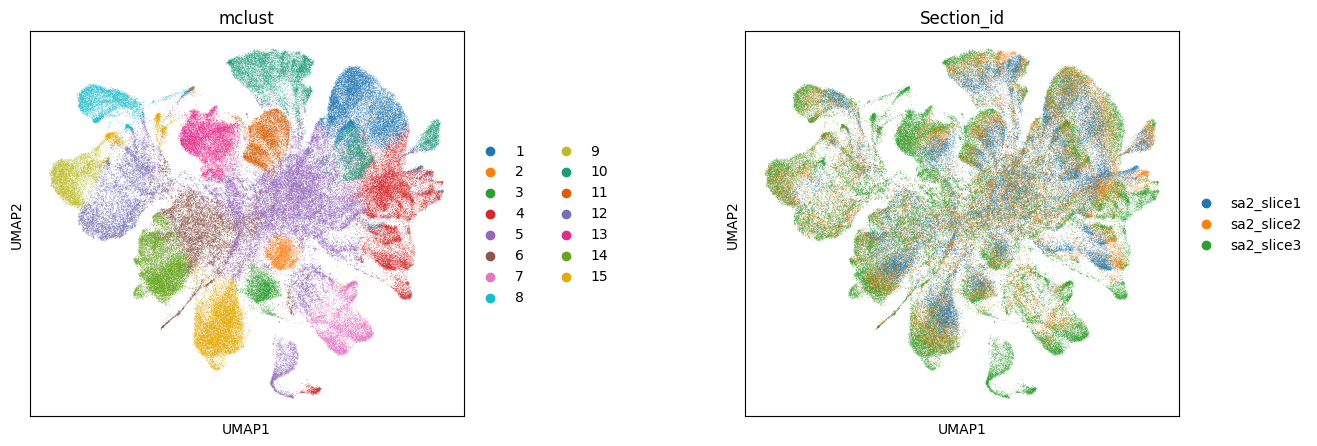
# Calculate FlatST features and run UMAP embedding based on the FlatST features extracted
sc.pp.neighbors(adata, use_rep='FlatST')
sc.tl.umap(adata)

# Set figure size
plt.rcParams["figure.figsize"] = (5, 5)

# Plot UMAP embedding with color by mclust and Section_id
sc.pl.umap(adata, color=['mclust', 'Section_id'], wspace=0.5)

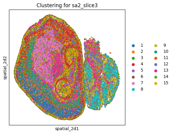
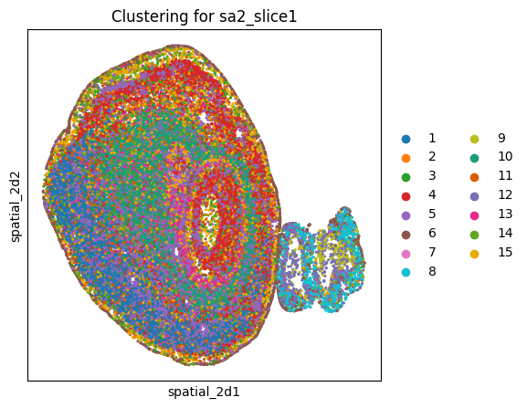
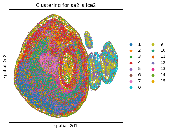
# Store spatial coordinates in obsm for scanpy plotting
adata.obsm['spatial_2d'] = adata.obs[['X', 'Y']].values

# Get all slice IDs
slices = adata.obs['Section_id'].unique()

for slice_id in slices:
    # Extract data for each slice
    adata_sub = adata[adata.obs['Section_id'] == slice_id].copy()

    # Plot clustering results for each slice
    sc.pl.embedding(adata_sub, basis='spatial_2d', color='mclust',
                    title=f'Clustering for {slice_id}',
                    size=20, show=True)